Demo of SNPmanifold
[ ]:
# If you want to use cuda

import torch
torch.set_default_device('cuda')
torch.cuda.set_device('cuda:0')
[1]:
# This demo dataset is available at data/MKN45_filtered in this GitHub repository.
# Import SNPmanifold and create an object of the class SNP_VAE.
# Run 1. filtering, 2. training, 3. clustering, 4. phylogeny in order.
# Each step can rerun sperately without reruning prior steps.

import SNPmanifold

# demo1 = SNPmanifold.SNP_VAE(path = "../../../../MKN45_filtered") <- output path of cellSNP-lite
# demo1 = SNPmanifold.SNP_VAE(AD = "cellSNP.tag.AD.mtx", DP = "cellSNP.tag.DP.mtx", VCF = "cellSNP.base.vcf.gz")
# demo1 = SNPmanifold.SNP_VAE(AD = "cellSNP.tag.AD.mtx", DP = "cellSNP.tag.DP.mtx", variant_name = "variant_name.tsv")

demo1 = SNPmanifold.SNP_VAE(AD = "/home/u3570318/mount2/SNPmanifold/data/MKN45_filtered/cellSNP.tag.AD.mtx", DP = "/home/u3570318/mount2/SNPmanifold/data/MKN45_filtered/cellSNP.tag.DP.mtx", variant_name = "/home/u3570318/mount2/SNPmanifold/data/MKN45_filtered/variant_name.tsv")
demo1.filtering()
demo1.training(is_cuda = True) # set is_cuda to False if you use CPU.
demo1.clustering(algorithm = "kmeans_umap3d", max_cluster = 20)
2024-05-29 04:51:57.969575: I tensorflow/stream_executor/platform/default/dso_loader.cc:49] Successfully opened dynamic library libcudart.so.10.1
Start loading raw data.
Finish loading raw data.
Start filtering low-quality cells and SNPs.
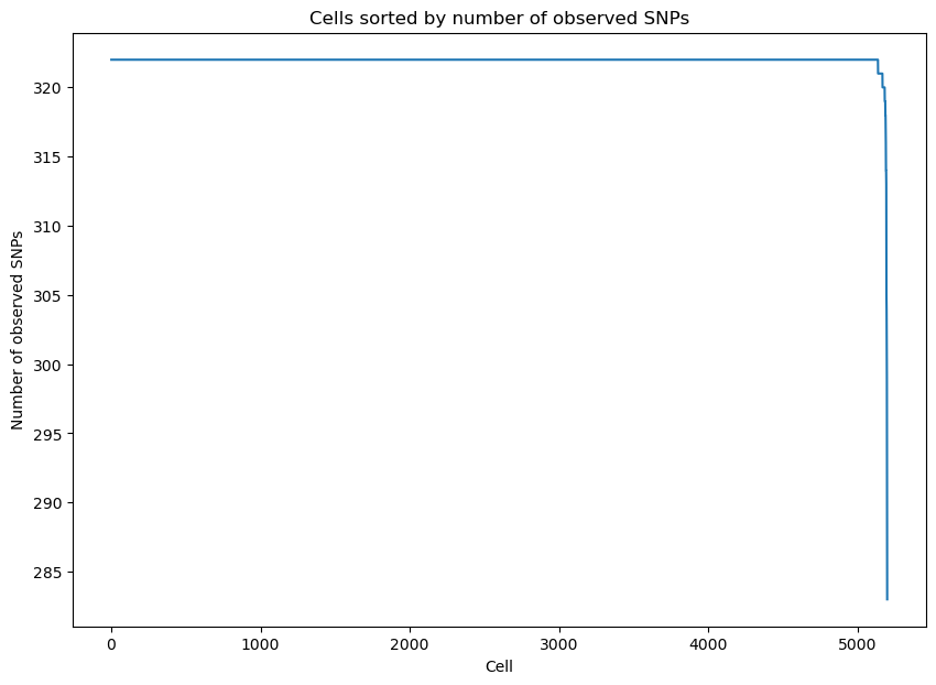
Please determine y-axis threshold in the plot to filter low-quality cells with low number of observed SNPs. 0
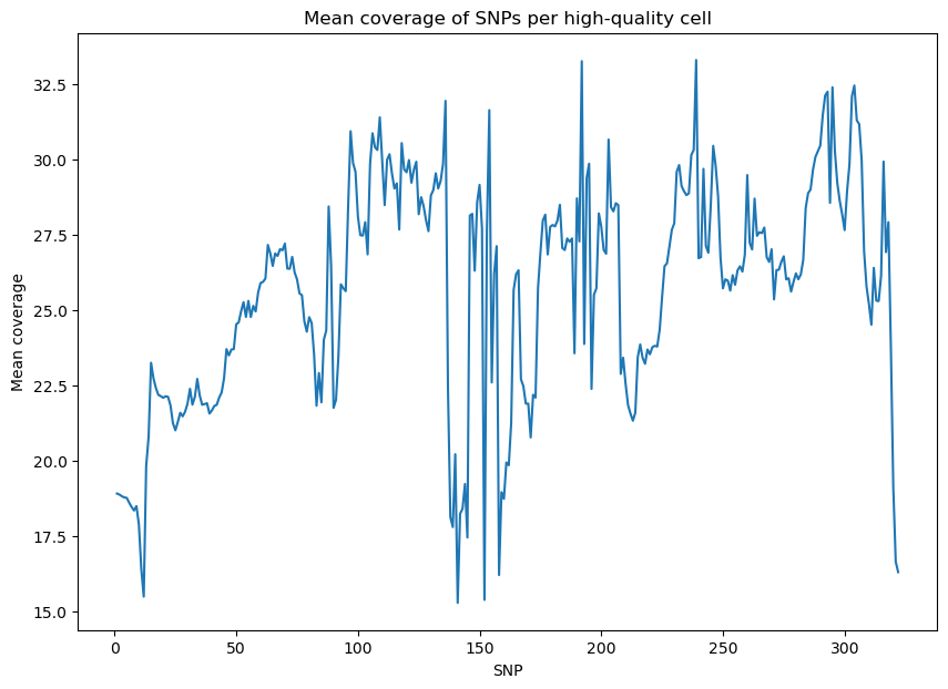
Please determine y-axis threshold in the plot to filter low-quality SNPs with low coverage. 0
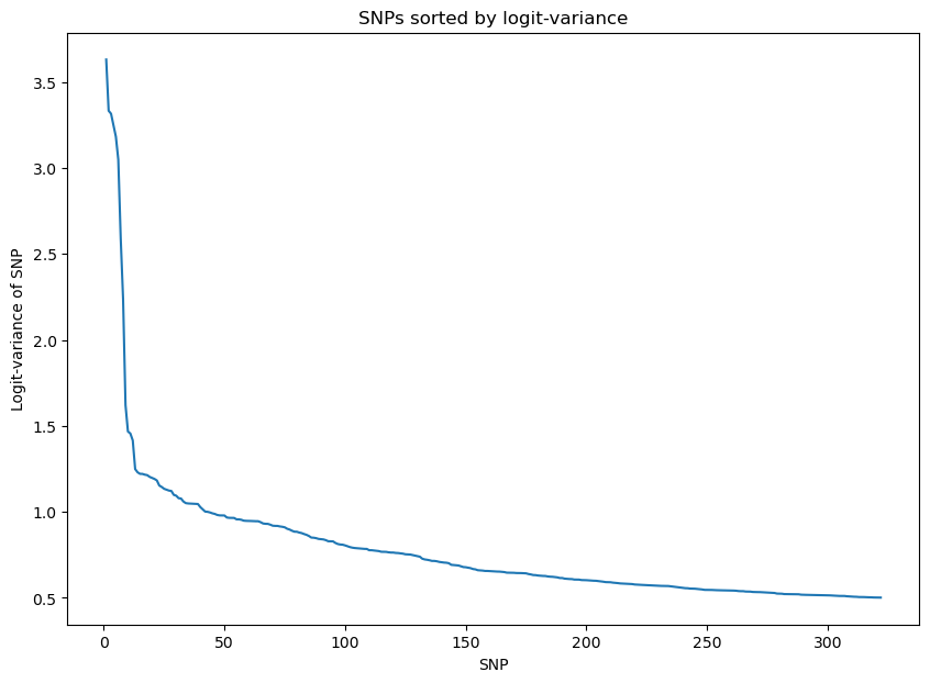
Please determine y-axis threshold in the plot to filter low-quality SNPs with low logit-variance. 0
Finish filtering low-quality data, 5199 cells and 322 SNPs will be used for downstream analysis.
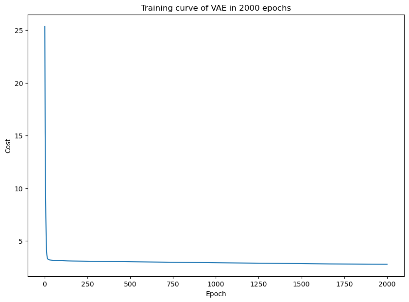
Start training VAE.
Epoch[10/2000], Cost: 4.655486
Epoch[20/2000], Cost: 3.267751
Epoch[30/2000], Cost: 3.202242
Epoch[40/2000], Cost: 3.183665
Epoch[50/2000], Cost: 3.170403
Epoch[60/2000], Cost: 3.161230
Epoch[70/2000], Cost: 3.151510
Epoch[80/2000], Cost: 3.143412
Epoch[90/2000], Cost: 3.136227
Epoch[100/2000], Cost: 3.129611
Epoch[200/2000], Cost: 3.093110
Epoch[300/2000], Cost: 3.071827
Epoch[400/2000], Cost: 3.052272
Epoch[500/2000], Cost: 3.032630
Epoch[600/2000], Cost: 3.013380
Epoch[700/2000], Cost: 2.994563
Epoch[800/2000], Cost: 2.975909
Epoch[900/2000], Cost: 2.957331
Epoch[1000/2000], Cost: 2.938742
Epoch[1100/2000], Cost: 2.920131
Epoch[1200/2000], Cost: 2.901630
Epoch[1300/2000], Cost: 2.883499
Epoch[1400/2000], Cost: 2.866161
Epoch[1500/2000], Cost: 2.849954
Epoch[1600/2000], Cost: 2.835345
Epoch[1700/2000], Cost: 2.822523
Epoch[1800/2000], Cost: 2.811750
Epoch[1900/2000], Cost: 2.803066
Epoch[2000/2000], Cost: 2.796290
Finish training VAE, training curve will be shown below.
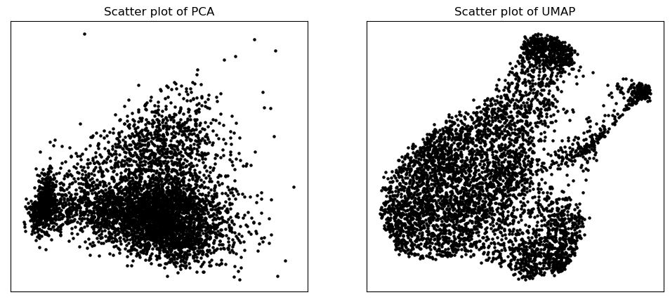
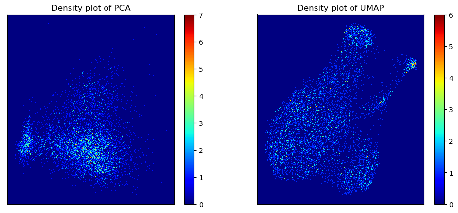
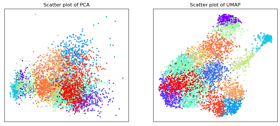
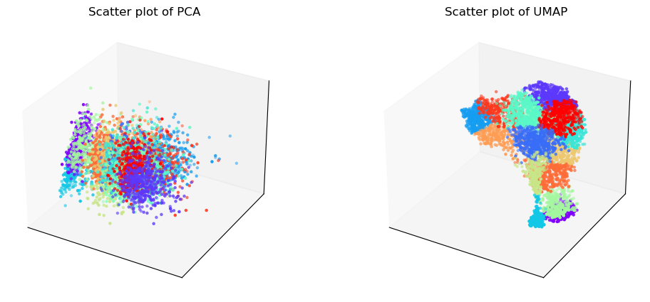
Start learning PCA and UMAP of latent space in VAE.
Finish learning, PCA and UMAP of latent space will be shown below.
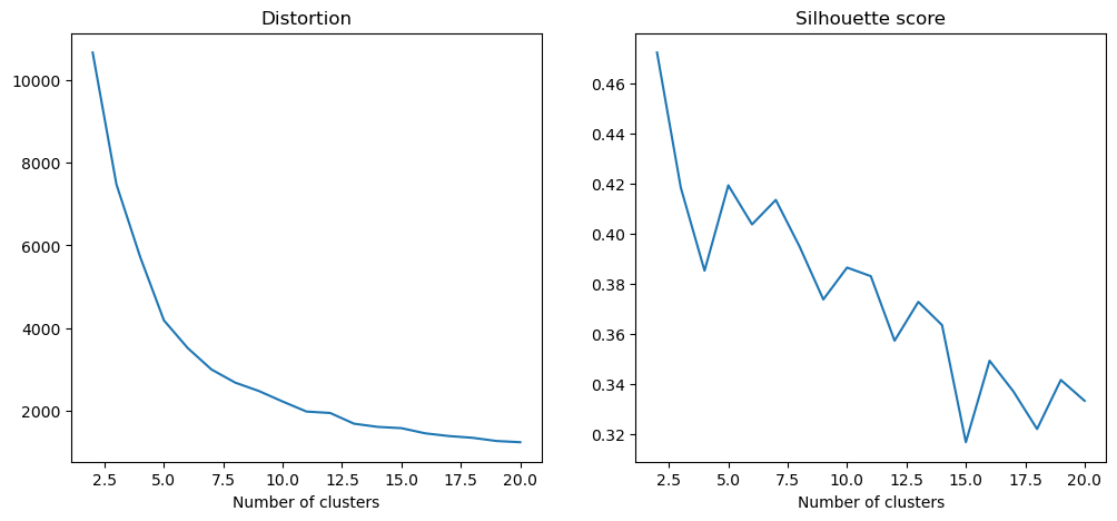
Start clustering.
2 clusters, Distortion: 10665.348633
3 clusters, Distortion: 7475.152832
4 clusters, Distortion: 5719.106445
5 clusters, Distortion: 4184.863770
6 clusters, Distortion: 3516.770996
7 clusters, Distortion: 2997.443848
8 clusters, Distortion: 2679.255859
9 clusters, Distortion: 2475.684570
10 clusters, Distortion: 2221.145020
11 clusters, Distortion: 1979.297119
12 clusters, Distortion: 1944.364014
13 clusters, Distortion: 1685.515137
14 clusters, Distortion: 1608.059326
15 clusters, Distortion: 1576.882080
16 clusters, Distortion: 1452.074219
17 clusters, Distortion: 1386.300171
18 clusters, Distortion: 1343.507324
19 clusters, Distortion: 1266.687256
20 clusters, Distortion: 1237.325684
Finish clustering, PCA, UMAP, distortion, silhouette score of K-means clustering will be shown below.


[2]:
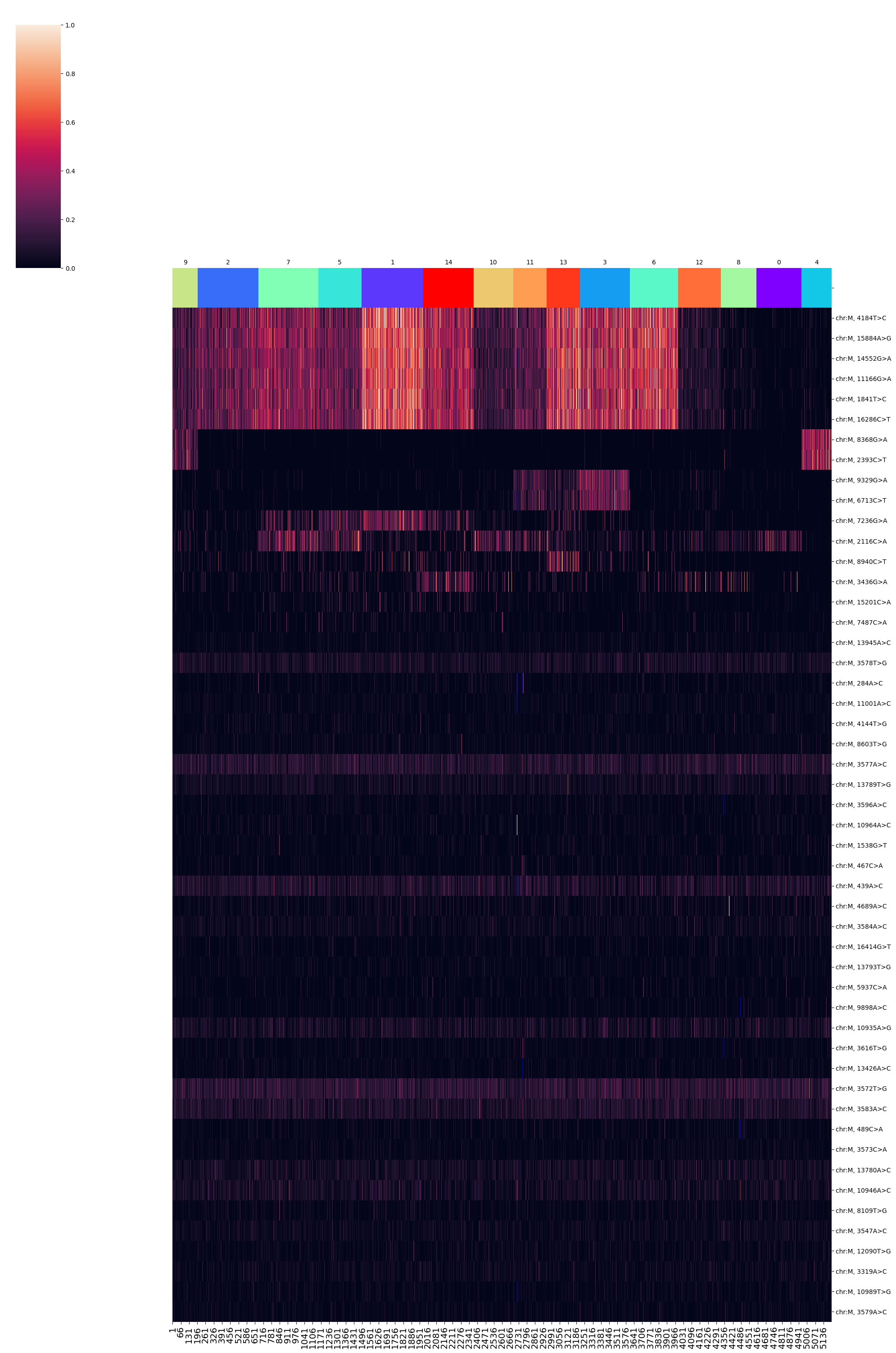
demo1.phylogeny(15) # number of clusters for downstream analysis
PCA and UMAP of individual clusters will be shown below.


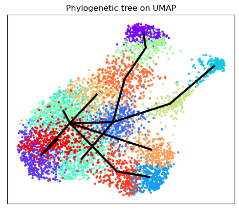
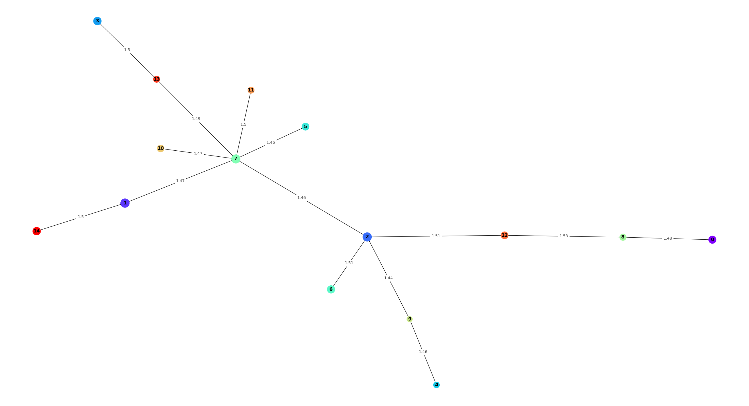
Phylogenetic tree in latent space will be shown below.
SNP-allelic ratios of 5199 cells and 50 SNPs will be shown below.
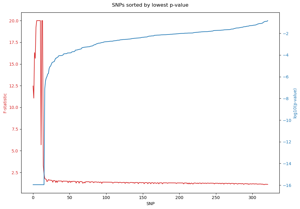
SNPs sorted by lowest p-value will be shown below
[ ]:
# Re-display figures in higher dpi

demo1.filtering_summary(dpi = 300)
demo1.training_summary(dpi = 300)
demo1.clustering_summary(dpi = 300)
demo1.phylogeny_summary(dpi = 300)
[3]:
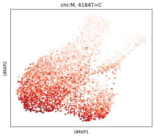
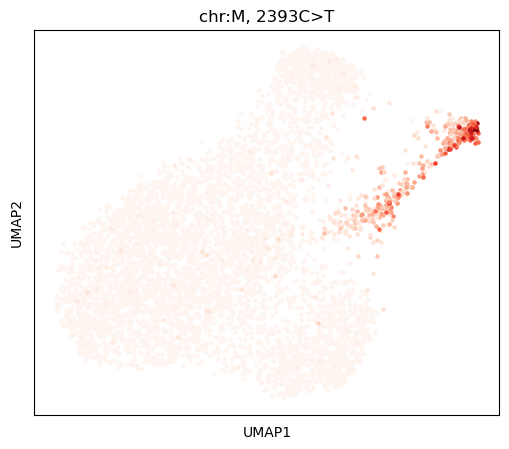
# Visualize frequency of particular SNPs on embeddings learnt by SNPmanifold

demo1.AF_scatter("chr:M, 4184T>C", dpi = 100)
demo1.AF_scatter("chr:M, 2393C>T", dpi = 100)
demo1.AF_scatter("chr:M, 9329G>A", dpi = 100)

[4]:
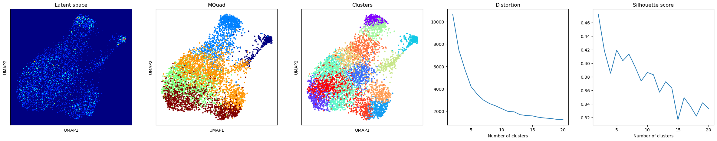
# Visualize cell labels assigned by another tool MQuad on embeddings learnt by SNPmanifold

import numpy as np
import matplotlib.cm as cm
import matplotlib.pyplot as plt

filter_mkn45 = np.genfromtxt('/home/u3570318/mount2/SNPmanifold/data/MKN45_filtered/cell_filter.csv').astype(bool)
df = np.genfromtxt('/home/u3570318/mount2/SNPmanifold/data/MKN45_filtered/id.csv', delimiter = ',')[filter_mkn45]

donors = []

for h in range(5):

    donors.append(np.where(df == h)[0])

fig, axs = plt.subplots(1, 5)
fig.set_size_inches(30, 5)

colors = cm.jet(np.linspace(0, 1, 5))

axs[1].set_title("MQuad")

for w in range(5):

    axs[1].scatter(demo1.embedding_2d[donors[w], 0], demo1.embedding_2d[donors[w], 1], s = 5, color = colors[w])

axs[1].set_xticks([])
axs[1].set_yticks([])
axs[1].set_xlabel("UMAP1")
axs[1].set_ylabel("UMAP2")

axs[0].hist2d(demo1.embedding_2d[:, 0], demo1.embedding_2d[:, 1], bins = (200, 200), cmap = plt.cm.jet \
              , range = np.array([demo1.xlim_embedding_2d, demo1.ylim_embedding_2d]))
axs[0].set_xticks([])
axs[0].set_yticks([])
axs[0].set_title("Latent space")
axs[0].set_xlabel("UMAP1")
axs[0].set_ylabel("UMAP2")

axs[2].set_title("Clusters")

for w in range(15):

    axs[2].scatter(demo1.embedding_2d[demo1.clusters[w], 0], demo1.embedding_2d[demo1.clusters[w], 1] \
                   , s = 5, color = demo1.colors[w])

axs[2].set_xticks([])
axs[2].set_yticks([])
axs[2].set_xlabel("UMAP1")
axs[2].set_ylabel("UMAP2")

axs[3].plot(np.arange(2, 21), demo1.distortions)
axs[3].set_title("Distortion")
axs[3].set_xlabel("Number of clusters")
axs[3].set_xticks([5, 10, 15, 20])
axs[4].set_title("Silhouette score")
axs[4].set_xlabel("Number of clusters")
axs[4].set_xticks([5, 10, 15, 20])
axs[4].plot(np.arange(2, 21), demo1.scores)

plt.show()